98 KiB
Chapter 4: Granger Causality Test
In the first three chapters, we discussed the classical methods for both univariate and multivariate time series forecasting. We now introduce the notion of causality and its implications on time series analysis in general. We also describe a test for the linear VAR model discussed in the previous chapter.
Prepared by: Carlo Vincienzo G. Dajac
Chapter Outline
Notations
Definitions
Assunmptions
Testing for Granger Causality
Notations
If \(A_t\) is a stationary stochastic process, let \(\overline A_t\) represent the set of past values \({A_{t-j}, \; j=1,2,\ldots,\infty}\) and \(\overline{\overline A}_t\) represent the set of past and present values \({A_{t-j}, \; j=0,1,\ldots,\infty}\). Further, let \(\overline A(k)\) represent the set \({A_{t-j}, \; j=k,k+1,\ldots,\infty}\).
Denote the optimum, unbiased, least-squares predictor of \(A_t\) using the set of values \(B_t\) by \(P_t (A|B)\). Thus, for instance, \(P_t (X|\overline X)\) will be the optimum predictor of \(X_t\) using only past \(X_t\). The predictive error series will be denoted by \(\varepsilon_t(A|B) = A_t - P_t(A|B)\). Let \(\sigma^2 (A|B)\) be the variance of \(\varepsilon_t(A|B)\).
Let \(U_t\) be all the information in the universe accumulated since time \(t-1\) and let \(U_t - Y_t\) denote all this information apart from the specified series \(Y_t\).
Definitions
Causality
If \(\sigma^2 (X|U) < \sigma^2 (X| \overline{U-Y})\), we say that \(Y\) is causing \(X\), denoted by \(Y_t \implies X_t\). We say that \(Y_t\) is causing \(X_t\) if we are able to predict \(X_t\) using all available information than if the information apart from \(Y_t\) had been used.
Feedback
If \(\sigma^2 (X|\overline U) < \sigma^2 (X| \overline{U-Y})\) and \(\sigma^2 (Y|\overline U) < \sigma^2 (Y| \overline{U-X})\), we say that feedback is occurring, which is denoted by \(Y_t \iff X_t\), i.e., feedback is said to occur when \(X_t\) is causing \(Y_t\) and also \(Y_t\) is causing \(X_t\).
Instantaneous Causality
If \(\sigma^2 (X|\overline U, \overline{\overline Y}) < \sigma^2 (X| \overline U)\), we say that instantaneous causality \(Y_t \implies X_t\) is occurring. In other words, the current value of \(X_t\) is better “predicted” if the present value of \(Y_t\) is included in the “prediction” than if it is not.
Causality Lag
If \(Y_t \implies X_t\), we define the (integer) causality lag \(m\) to be the least value of \(k\) such that \(\sigma^2 (X|U-Y(k)) < \sigma^2 (X|U-Y(k+1))\). Thus, knowing the values \(Y_{t-j}, \; j=0,1,\ldots,m-1\) will be of no help in improving the prediction of \(X_t\)
Assumptions
Series is stationary.
Linear model is already optimized.
Testing for Granger Causality
import pandas as pd
import numpy as np
import matplotlib.pyplot as plt
from scipy import stats
from pandas.plotting import lag_plot
from statsmodels.tsa.api import VAR
from statsmodels.tsa.stattools import adfuller
from statsmodels.tsa.stattools import kpss
from statsmodels.tsa.stattools import grangercausalitytests
from statsmodels.tools.eval_measures import rmse, aic
from statsmodels.stats.stattools import durbin_watson
We will use the Ipo dataset in this notebook.
data = pd.read_csv('../data/Ipo_dataset.csv', index_col='Time');
data = data.dropna()
data
| Rain | ONI | NIA | Dam | |
|---|---|---|---|---|
| Time | ||||
| 0 | 0.00 | -0.7 | 38.225693 | 100.70 |
| 1 | 0.00 | -0.7 | 57.996530 | 100.63 |
| 2 | 0.00 | -0.7 | 49.119213 | 100.56 |
| 3 | 0.00 | -0.7 | 47.034720 | 100.55 |
| 4 | 0.00 | -0.7 | 42.223380 | 100.48 |
| ... | ... | ... | ... | ... |
| 7111 | 1.80 | -0.2 | 5.040000 | 100.86 |
| 7112 | 1.60 | -0.2 | 4.500000 | 101.01 |
| 7113 | 21.60 | -0.2 | 6.730000 | 101.08 |
| 7114 | 0.20 | -0.2 | 6.720000 | 100.92 |
| 7115 | 46.82 | -0.2 | 1.950000 | 100.97 |
7116 rows × 4 columns
As an example, we will only use the NIA and Dam time series.
data = data.drop(['NIA', 'ONI'], axis=1)
data
| Rain | Dam | |
|---|---|---|
| Time | ||
| 0 | 0.00 | 100.70 |
| 1 | 0.00 | 100.63 |
| 2 | 0.00 | 100.56 |
| 3 | 0.00 | 100.55 |
| 4 | 0.00 | 100.48 |
| ... | ... | ... |
| 7111 | 1.80 | 100.86 |
| 7112 | 1.60 | 101.01 |
| 7113 | 21.60 | 101.08 |
| 7114 | 0.20 | 100.92 |
| 7115 | 46.82 | 100.97 |
7116 rows × 2 columns
Step 1: Test each time series for stationarity. Ideally, this should involve using a test (such as the ADF test) where the null hypothesis is non-stationarity, as well as a test (such as the KPSS test) where the null is stationarity. This is a good cross-check.
f2, (ax4, ax5) = plt.subplots(1, 2, figsize=(15, 5))
f2.tight_layout()

lag_plot(data['Rain'], ax=ax4)
ax4.set_title('Rainfall');

# lag_plot(data['NIA'], ax=ax4)
# ax4.set_title('NIA Releases');

lag_plot(data['Dam'], ax=ax5)
ax5.set_title('Dam Water Level');

plt.show()
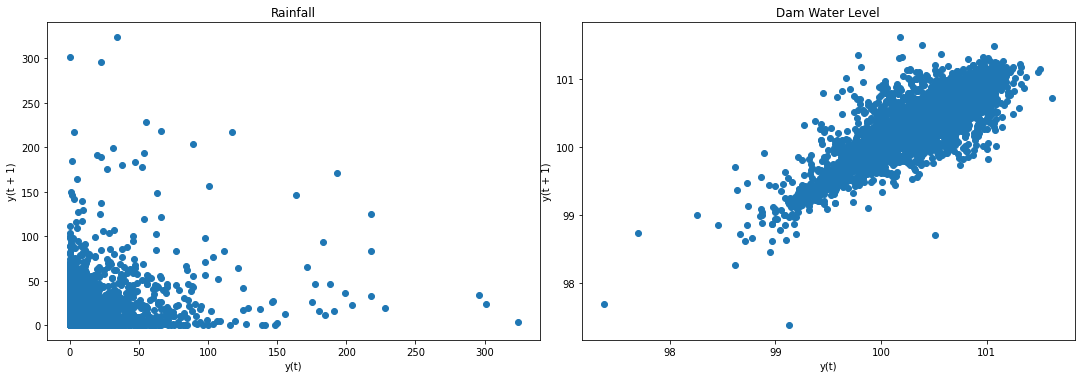
Result: Both data are not stationary. We can make them stationary through differencing.
# differencing for stationarity check
rawData = data.copy(deep=True)

# data['Rain'] = data['Rain'] - data['Rain'].shift(1)
# data['NIA'] = data['NIA'] - data['NIA'].shift(1)
data['Dam'] = data['Dam'] - data['Dam'].shift(1)
data = data.dropna()
# split data into train and test sets for VAR later on
end = round(len(data)*.8)
train = data[:end]
test = data[end:]
# ADF Null Hypothesis: there is a unit root, meaning series is non-stationary

X1 = np.array(data['Dam'])
X1 = X1[~np.isnan(X1)]

result = adfuller(X1)
print('ADF Statistic: %f' % result[0])
print('p-value: %f' % result[1])
print('Critical Values:')
for key, value in result[4].items():
    print('\t%s: %.3f' % (key, value))


X2 = np.array(data['Rain'])
# X2 = np.array(data['NIA'])
X2 = X2[~np.isnan(X2)]

result = adfuller(X2)
print('ADF Statistic: %f' % result[0])
print('p-value: %f' % result[1])
print('Critical Values:')
for key, value in result[4].items():
    print('\t%s: %.3f' % (key, value))
ADF Statistic: -21.591918
p-value: 0.000000
Critical Values:
	1%: -3.431
	5%: -2.862
	10%: -2.567
ADF Statistic: -8.622738
p-value: 0.000000
Critical Values:
	1%: -3.431
	5%: -2.862
	10%: -2.567
# KPSS Null Hypothesis: there is no unit root, meaning series is stationary

def kpss_test(series, **kw):
    statistic, p_value, n_lags, critical_values = kpss(series, **kw)
    # Format Output
    print(f'KPSS Statistic: {statistic}')
    print(f'p-value: {p_value}')
    print(f'num lags: {n_lags}')
    print('Critial Values:')
    for key, value in critical_values.items():
        print(f'   {key} : {value}')
    print(f'Result: The series is {"not " if p_value < 0.05 else ""}stationary')

kpss_test(X1)
kpss_test(X2)
KPSS Statistic: 0.009242367643647224
p-value: 0.1
num lags: 35
Critial Values:
   10% : 0.347
   5% : 0.463
   2.5% : 0.574
   1% : 0.739
Result: The series is stationary
KPSS Statistic: 0.09395749653745288
p-value: 0.1
num lags: 35
Critial Values:
   10% : 0.347
   5% : 0.463
   2.5% : 0.574
   1% : 0.739
Result: The series is stationary
/Users/prince.javier/opt/anaconda3/envs/atsa/lib/python3.7/site-packages/statsmodels/tsa/stattools.py:1875: FutureWarning: The behavior of using nlags=None will change in release 0.13.Currently nlags=None is the same as nlags="legacy", and so a sample-size lag length is used. After the next release, the default will change to be the same as nlags="auto" which uses an automatic lag length selection method. To silence this warning, either use "auto" or "legacy"
  warnings.warn(msg, FutureWarning)
/Users/prince.javier/opt/anaconda3/envs/atsa/lib/python3.7/site-packages/statsmodels/tsa/stattools.py:1911: InterpolationWarning: The test statistic is outside of the range of p-values available in the
look-up table. The actual p-value is greater than the p-value returned.

  warn_msg.format(direction="greater"), InterpolationWarning
Results: ADF Null Hypothesis is rejected. Thus, data is stationary. KPSS Null Hypothesis could not be rejected. Thus, data is stationary.
f2, (ax4, ax5) = plt.subplots(1, 2, figsize=(15, 5))
f2.tight_layout()

lag_plot(data['Rain'], ax=ax4)
ax4.set_title('Rainfall');

# lag_plot(data['NIA'], ax=ax4)
# ax4.set_title('NIA Releases');

lag_plot(data['Dam'], ax=ax5)
ax5.set_title('Dam Water Level');

plt.show()
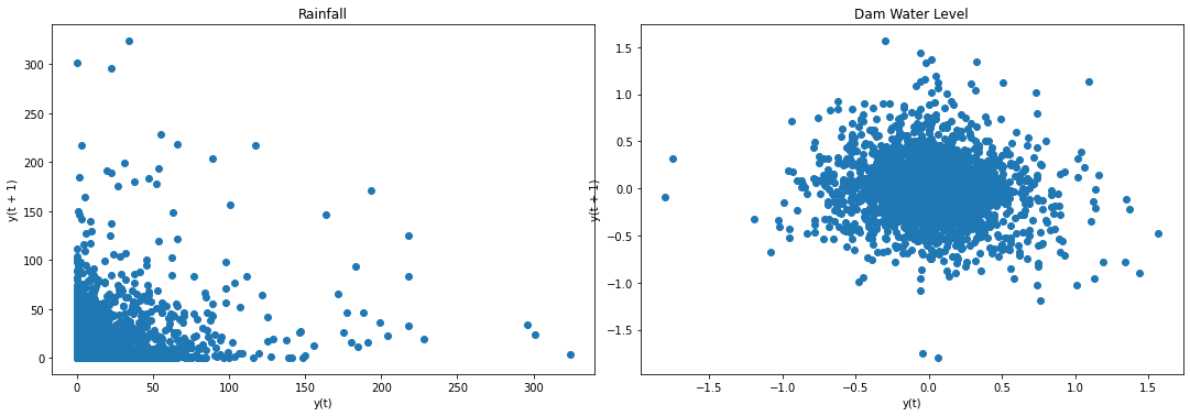
Result: Lag plots confirm results of ADF test and KPSS test.
Step 2: Set up a VAR model for the data (without differencing).
model = VAR(train)
model_fitted = model.fit(2)
/Users/prince.javier/opt/anaconda3/envs/atsa/lib/python3.7/site-packages/statsmodels/tsa/base/tsa_model.py:579: ValueWarning: An unsupported index was provided and will be ignored when e.g. forecasting.
  ' ignored when e.g. forecasting.', ValueWarning)
Step 4: Make sure that the VAR is well-specified. For example, ensure that there is no serial correlation in the residuals. If need be, increase p until any autocorrelation issues are resolved.
#Check for Serial Correlation of Residuals (Errors) using Durbin Watson Statistic
#The value of this statistic can vary between 0 and 4.
#The closer it is to the value 2, then there is no significant serial correlation.
#The closer to 0, there is a positive serial correlation,
#and the closer it is to 4 implies negative serial correlation.

out = durbin_watson(model_fitted.resid)

for col, val in zip(data.columns, out):
    print(col, ':', round(val, 2))
Rain : 2.01
Dam : 2.07
Result: There is no significant correlation between in the residuals.
Step 5: Now take the preferred VAR model and add in m additional lags of each of the variables into each of the equations.
model = VAR(train)
model_fitted = model.fit(2)
#get the lag order
lag_order = model_fitted.k_ar
print(lag_order)
2
/Users/prince.javier/opt/anaconda3/envs/atsa/lib/python3.7/site-packages/statsmodels/tsa/base/tsa_model.py:579: ValueWarning: An unsupported index was provided and will be ignored when e.g. forecasting.
  ' ignored when e.g. forecasting.', ValueWarning)
Step 6: Test for Granger non-causality.
maxlag = lag_order
test = 'ssr_chi2test'
def grangers_causation_matrix(data, variables, test='ssr_chi2test', verbose=False):
    """Check Granger Causality of all possible combinations of the time series.
    The rows are the response variable, columns are predictors. The values in the table
    are the P-Values. P-Values lesser than the significance level (0.05), implies
    the Null Hypothesis that the coefficients of the corresponding past values is
    zero, that is, the X does not cause Y can be rejected.

    data      : pandas dataframe containing the time series variables
    variables : list containing names of the time series variables.
    """
    df = pd.DataFrame(np.zeros((len(variables), len(variables))), columns=variables, index=variables)
    for c in df.columns:
        for r in df.index:
            test_result = grangercausalitytests(data[[r, c]], maxlag=maxlag, verbose=False)
            p_values = [round(test_result[i+1][0][test][1],4) for i in range(maxlag)]
            if verbose: print(f'Y = {r}, X = {c}, P Values = {p_values}')
            min_p_value = np.min(p_values)
            df.loc[r, c] = min_p_value
    df.columns = [var + '_x' for var in variables]
    df.index = [var + '_y' for var in variables]
    return df

o = grangers_causation_matrix(train, variables = train.columns)
o
| Rain_x | Dam_x | |
|---|---|---|
| Rain_y | 1.0 | 0.2932 |
| Dam_y | 0.0 | 1.0000 |
Result: If a given p-value is < significance level (0.05), then, the corresponding X series (column) causes the Y (row).
For this particular example, we can say that NIA releases causes changes in the dam water level. On the other hand, dam water level also causes changes in the NIA releases. This is an example of the feedback mentioned above.
We do the similar steps for the La Mesa dataset.
data = pd.read_csv('../data/La Mesa_dataset.csv', index_col='Time');
data = data.dropna()
data = data.drop(['Rain', 'ONI'], axis=1)
# data['Rain'] = data['Rain'] - data['Rain'].shift(1)
data['NIA'] = data['NIA'] - data['NIA'].shift(1)
data['Dam'] = data['Dam'] - data['Dam'].shift(1)
data = data.dropna()

train = data[:end]
test = data[end:]

model = VAR(train)
model_fitted = model.fit(2)
lag_order = model_fitted.k_ar

maxlag = lag_order
test = 'ssr_chi2test'

o1 = grangers_causation_matrix(train, variables = train.columns)
o1
/Users/prince.javier/opt/anaconda3/envs/atsa/lib/python3.7/site-packages/statsmodels/tsa/base/tsa_model.py:579: ValueWarning: An unsupported index was provided and will be ignored when e.g. forecasting.
  ' ignored when e.g. forecasting.', ValueWarning)
| NIA_x | Dam_x | |
|---|---|---|
| NIA_y | 1.000 | 0.1632 |
| Dam_y | 0.636 | 1.0000 |
We see that, unlike for Ipo, NIA releases and dam water level are NOT causal to one another.
Exercises
As exercises, the reader can check for causality between other pairs of variables from both the Ipo and La Mesa datasets, as well as from the Angat dataset.
Jena Weather Data
We look back at the Jena Weather Data and explore which variables are causal to one another.
jena_data = pd.read_csv('../data/jena_climate_2009_2016.csv')
jena_data['Date Time'] = pd.to_datetime(jena_data['Date Time'])
jena_data = jena_data.set_index('Date Time')
jena_data.head(3)
| p (mbar) | T (degC) | Tpot (K) | Tdew (degC) | rh (%) | VPmax (mbar) | VPact (mbar) | VPdef (mbar) | sh (g/kg) | H2OC (mmol/mol) | rho (g/m**3) | wv (m/s) | max. wv (m/s) | wd (deg) | |
|---|---|---|---|---|---|---|---|---|---|---|---|---|---|---|
| Date Time | ||||||||||||||
| 2009-01-01 00:10:00 | 996.52 | -8.02 | 265.40 | -8.90 | 93.3 | 3.33 | 3.11 | 0.22 | 1.94 | 3.12 | 1307.75 | 1.03 | 1.75 | 152.3 |
| 2009-01-01 00:20:00 | 996.57 | -8.41 | 265.01 | -9.28 | 93.4 | 3.23 | 3.02 | 0.21 | 1.89 | 3.03 | 1309.80 | 0.72 | 1.50 | 136.1 |
| 2009-01-01 00:30:00 | 996.53 | -8.51 | 264.91 | -9.31 | 93.9 | 3.21 | 3.01 | 0.20 | 1.88 | 3.02 | 1310.24 | 0.19 | 0.63 | 171.6 |
Consider last 10,000 data points for p and T.
jena_sample = jena_data.iloc[:,:2]
jena_sample.head(3)
| p (mbar) | T (degC) | |
|---|---|---|
| Date Time | ||
| 2009-01-01 00:10:00 | 996.52 | -8.02 |
| 2009-01-01 00:20:00 | 996.57 | -8.41 |
| 2009-01-01 00:30:00 | 996.53 | -8.51 |
f2, (ax4, ax5) = plt.subplots(1, 2, figsize=(15, 5))
f2.tight_layout()

lag_plot(jena_sample['p (mbar)'], ax=ax4)
ax4.set_title('p (mbar)');

lag_plot(jena_sample['T (degC)'], ax=ax5)
ax5.set_title('T (degC)');

plt.show()
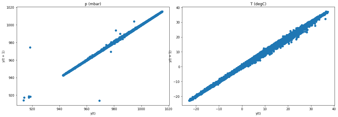
Result: T data is not stationary. We use differencing to make it stationary.
# differencing for stationarity check
rawData = jena_sample.copy(deep=True)

jena_sample['p (mbar)'] = jena_sample['p (mbar)'] - jena_sample['p (mbar)'].shift(1)
jena_sample['T (degC)'] = jena_sample['T (degC)'] - jena_sample['T (degC)'].shift(1)
jena_sample = jena_sample.dropna()
<ipython-input-98-3aed1e4c60a7>:4: SettingWithCopyWarning:
A value is trying to be set on a copy of a slice from a DataFrame.
Try using .loc[row_indexer,col_indexer] = value instead

See the caveats in the documentation: https://pandas.pydata.org/pandas-docs/stable/user_guide/indexing.html#returning-a-view-versus-a-copy
  jena_sample['p (mbar)'] = jena_sample['p (mbar)'] - jena_sample['p (mbar)'].shift(1)
<ipython-input-98-3aed1e4c60a7>:5: SettingWithCopyWarning:
A value is trying to be set on a copy of a slice from a DataFrame.
Try using .loc[row_indexer,col_indexer] = value instead

See the caveats in the documentation: https://pandas.pydata.org/pandas-docs/stable/user_guide/indexing.html#returning-a-view-versus-a-copy
  jena_sample['T (degC)'] = jena_sample['T (degC)'] - jena_sample['T (degC)'].shift(1)
# split data into train and test sets for VAR later on
end = round(len(jena_sample)*.8)
train = jena_sample[:end]
test = jena_sample[end:]
# ADF Null Hypothesis: there is a unit root, meaning series is non-stationary

X1 = np.array(jena_sample['p (mbar)'])
X1 = X1[~np.isnan(X1)]

result = adfuller(X1)
print('ADF Statistic: %f' % result[0])
print('p-value: %f' % result[1])
print('Critical Values:')
for key, value in result[4].items():
    print('\t%s: %.3f' % (key, value))


X2 = np.array(jena_sample['T (degC)'])
X2 = X2[~np.isnan(X2)]

result = adfuller(X2)
print('ADF Statistic: %f' % result[0])
print('p-value: %f' % result[1])
print('Critical Values:')
for key, value in result[4].items():
    print('\t%s: %.3f' % (key, value))
ADF Statistic: -59.104716
p-value: 0.000000
Critical Values:
	1%: -3.430
	5%: -2.862
	10%: -2.567
ADF Statistic: -122.256393
p-value: 0.000000
Critical Values:
	1%: -3.430
	5%: -2.862
	10%: -2.567
# KPSS Null Hypothesis: there is no unit root, meaning series is stationary

def kpss_test(series, **kw):
    statistic, p_value, n_lags, critical_values = kpss(series, **kw)
    # Format Output
    print(f'KPSS Statistic: {statistic}')
    print(f'p-value: {p_value}')
    print(f'num lags: {n_lags}')
    print('Critial Values:')
    for key, value in critical_values.items():
        print(f'   {key} : {value}')
    print(f'Result: The series is {"not " if p_value < 0.05 else ""}stationary')

kpss_test(X1)
kpss_test(X2)
KPSS Statistic: 0.0016032868205162105
p-value: 0.1
num lags: 97
Critial Values:
   10% : 0.347
   5% : 0.463
   2.5% : 0.574
   1% : 0.739
Result: The series is stationary
KPSS Statistic: 0.002692749007731491
p-value: 0.1
num lags: 97
Critial Values:
   10% : 0.347
   5% : 0.463
   2.5% : 0.574
   1% : 0.739
Result: The series is stationary
/opt/conda/lib/python3.8/site-packages/statsmodels/tsa/stattools.py:1850: FutureWarning: The behavior of using nlags=None will change in release 0.13.Currently nlags=None is the same as nlags="legacy", and so a sample-size lag length is used. After the next release, the default will change to be the same as nlags="auto" which uses an automatic lag length selection method. To silence this warning, either use "auto" or "legacy"
  warnings.warn(msg, FutureWarning)
/opt/conda/lib/python3.8/site-packages/statsmodels/tsa/stattools.py:1885: InterpolationWarning: The test statistic is outside of the range of p-values available in the
look-up table. The actual p-value is greater than the p-value returned.

  warnings.warn(
/opt/conda/lib/python3.8/site-packages/statsmodels/tsa/stattools.py:1885: InterpolationWarning: The test statistic is outside of the range of p-values available in the
look-up table. The actual p-value is greater than the p-value returned.

  warnings.warn(
Results: ADF Null Hypothesis is rejected. Thus, data is stationary. KPSS Null Hypothesis could not be rejected. Thus, data is stationary.
f2, (ax4, ax5) = plt.subplots(1, 2, figsize=(15, 5))
f2.tight_layout()

lag_plot(jena_sample['p (mbar)'], ax=ax4)
ax4.set_title('p (mbar)');

lag_plot(jena_sample['T (degC)'], ax=ax5)
ax5.set_title('T (degC)');

plt.show()
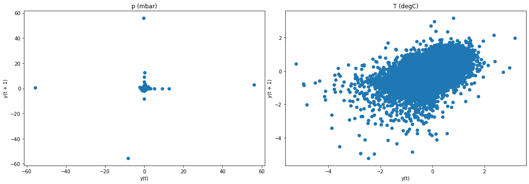
Result: Lag plots confirm results of ADF test and KPSS test.
Step 2: Set up a VAR model for the data (without differencing).
model = VAR(train)
model_fitted = model.fit(2)
/opt/conda/lib/python3.8/site-packages/statsmodels/tsa/base/tsa_model.py:581: ValueWarning: A date index has been provided, but it has no associated frequency information and so will be ignored when e.g. forecasting.
  warnings.warn('A date index has been provided, but it has no'
/opt/conda/lib/python3.8/site-packages/statsmodels/tsa/base/tsa_model.py:585: ValueWarning: A date index has been provided, but it is not monotonic and so will be ignored when e.g. forecasting.
  warnings.warn('A date index has been provided, but it is not'
Step 4: Make sure that the VAR is well-specified. For example, ensure that there is no serial correlation in the residuals. If need be, increase p until any autocorrelation issues are resolved.
#Check for Serial Correlation of Residuals (Errors) using Durbin Watson Statistic
#The value of this statistic can vary between 0 and 4.
#The closer it is to the value 2, then there is no significant serial correlation.
#The closer to 0, there is a positive serial correlation,
#and the closer it is to 4 implies negative serial correlation.

out = durbin_watson(model_fitted.resid)

for col, val in zip(data.columns, out):
    print(col, ':', round(val, 2))
Rain : 2.01
Dam : 2.0
Result: There is no significant correlation between in the residuals.
Step 5: Now take the preferred VAR model and add in m additional lags of each of the variables into each of the equations.
model = VAR(train)
model_fitted = model.fit(2)
#get the lag order
lag_order = model_fitted.k_ar
print(lag_order)
/opt/conda/lib/python3.8/site-packages/statsmodels/tsa/base/tsa_model.py:581: ValueWarning: A date index has been provided, but it has no associated frequency information and so will be ignored when e.g. forecasting.
  warnings.warn('A date index has been provided, but it has no'
/opt/conda/lib/python3.8/site-packages/statsmodels/tsa/base/tsa_model.py:585: ValueWarning: A date index has been provided, but it is not monotonic and so will be ignored when e.g. forecasting.
  warnings.warn('A date index has been provided, but it is not'
2
Step 6: Test for Granger non-causality.
maxlag = lag_order
test = 'ssr_chi2test'
def grangers_causation_matrix(data, variables, test='ssr_chi2test', verbose=False):
    """Check Granger Causality of all possible combinations of the time series.
    The rows are the response variable, columns are predictors. The values in the table
    are the P-Values. P-Values lesser than the significance level (0.05), implies
    the Null Hypothesis that the coefficients of the corresponding past values is
    zero, that is, the X does not cause Y can be rejected.

    data      : pandas dataframe containing the time series variables
    variables : list containing names of the time series variables.
    """
    df = pd.DataFrame(np.zeros((len(variables), len(variables))), columns=variables, index=variables)
    for c in df.columns:
        for r in df.index:
            test_result = grangercausalitytests(data[[r, c]], maxlag=maxlag, verbose=False)
            p_values = [round(test_result[i+1][0][test][1],4) for i in range(maxlag)]
            if verbose: print(f'Y = {r}, X = {c}, P Values = {p_values}')
            min_p_value = np.min(p_values)
            df.loc[r, c] = min_p_value
    df.columns = [var + '_x' for var in variables]
    df.index = [var + '_y' for var in variables]
    return df

o = grangers_causation_matrix(train, variables = train.columns)
o
| p (mbar)_x | T (degC)_x | |
|---|---|---|
| p (mbar)_y | 1.0 | 0.0 |
| T (degC)_y | 0.0 | 1.0 |
We observe that p “causes” T, but not the other way around.
Causality will be revisited in a later chapter, in particular addressing the limitations of the method discussed in this chapter.
By students of PhD in Data Science Batch 2023 at the Asian Institute of Management
© Copyright 2020.