59 KiB

Raw Blame History

Temperature Forecasting (Supplementary Notebook)¶

Similar to what was done in previous sections, this notebook applies the methodology used in the M5 Forecasting notebook to the Jena Climate dataset. Specifically, we will be forecasting the temperature variable.

1. Jena Climate Dataset¶

Let’s load the dataset and examine it.

import numpy as np
import pandas as pd
import matplotlib.pyplot as plt

### CREATE X,Y ####
def create_xy(series, window_size, prediction_horizon, shuffle = False):
    x = []
    y = []
    for i in range(0, len(series)):
        if len(series[(i + window_size):(i + window_size + prediction_horizon)]) < prediction_horizon:
            break
        x.append(series[i:(i + window_size)])
        y.append(series[(i + window_size):(i + window_size + prediction_horizon)])
    x = np.array(x)
    y = np.array(y)
    return x,y

plt.rcParams['figure.figsize'] = [15, 5]

np.set_printoptions(precision = 6, suppress = True)

df = pd.read_csv('../data/jena_climate_2009_2016.csv')
df.shape

(420551, 15)

df.head(10)

	Date Time	p (mbar)	T (degC)	Tpot (K)	Tdew (degC)	rh (%)	VPmax (mbar)	VPact (mbar)	VPdef (mbar)	sh (g/kg)	H2OC (mmol/mol)	rho (g/m**3)	wv (m/s)	max. wv (m/s)	wd (deg)
0	01.01.2009 00:10:00	996.52	-8.02	265.40	-8.90	93.3	3.33	3.11	0.22	1.94	3.12	1307.75	1.03	1.75	152.3
1	01.01.2009 00:20:00	996.57	-8.41	265.01	-9.28	93.4	3.23	3.02	0.21	1.89	3.03	1309.80	0.72	1.50	136.1
2	01.01.2009 00:30:00	996.53	-8.51	264.91	-9.31	93.9	3.21	3.01	0.20	1.88	3.02	1310.24	0.19	0.63	171.6
3	01.01.2009 00:40:00	996.51	-8.31	265.12	-9.07	94.2	3.26	3.07	0.19	1.92	3.08	1309.19	0.34	0.50	198.0
4	01.01.2009 00:50:00	996.51	-8.27	265.15	-9.04	94.1	3.27	3.08	0.19	1.92	3.09	1309.00	0.32	0.63	214.3
5	01.01.2009 01:00:00	996.50	-8.05	265.38	-8.78	94.4	3.33	3.14	0.19	1.96	3.15	1307.86	0.21	0.63	192.7
6	01.01.2009 01:10:00	996.50	-7.62	265.81	-8.30	94.8	3.44	3.26	0.18	2.04	3.27	1305.68	0.18	0.63	166.5
7	01.01.2009 01:20:00	996.50	-7.62	265.81	-8.36	94.4	3.44	3.25	0.19	2.03	3.26	1305.69	0.19	0.50	118.6
8	01.01.2009 01:30:00	996.50	-7.91	265.52	-8.73	93.8	3.36	3.15	0.21	1.97	3.16	1307.17	0.28	0.75	188.5
9	01.01.2009 01:40:00	996.53	-8.43	264.99	-9.34	93.1	3.23	3.00	0.22	1.88	3.02	1309.85	0.59	0.88	185.0

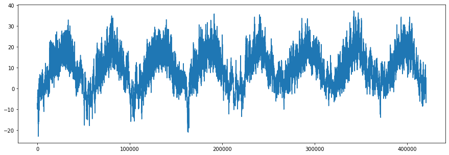
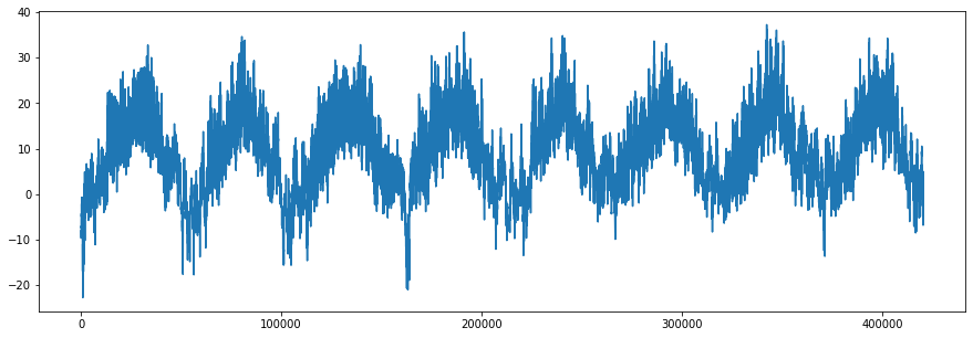
series = df['T (degC)'].iloc[5:]

series.plot()
plt.show()
print(series.shape)

../_images/lightgbm_jena_forecasting_4_0.png

(420546,)

series = series.iloc[::6]

series.plot()
plt.show()
print(series.shape)

../_images/lightgbm_jena_forecasting_5_0.png

(70091,)

series = df.iloc[::6, 1:]
series

	p (mbar)	T (degC)	Tpot (K)	Tdew (degC)	rh (%)	VPmax (mbar)	VPact (mbar)	VPdef (mbar)	sh (g/kg)	H2OC (mmol/mol)	rho (g/m**3)	wv (m/s)	max. wv (m/s)	wd (deg)
0	996.52	-8.02	265.40	-8.90	93.30	3.33	3.11	0.22	1.94	3.12	1307.75	1.03	1.75	152.3
6	996.50	-7.62	265.81	-8.30	94.80	3.44	3.26	0.18	2.04	3.27	1305.68	0.18	0.63	166.5
12	996.63	-8.85	264.57	-9.70	93.50	3.12	2.92	0.20	1.82	2.93	1312.11	0.16	0.50	158.3
18	996.87	-8.84	264.56	-9.69	93.50	3.13	2.92	0.20	1.83	2.93	1312.37	0.07	0.25	129.3
24	997.05	-9.23	264.15	-10.25	92.20	3.03	2.79	0.24	1.74	2.80	1314.62	0.10	0.38	203.9
...	...	...	...	...	...	...	...	...	...	...	...	...	...	...
420522	1002.08	-1.40	271.59	-6.10	70.20	5.51	3.87	1.64	2.40	3.86	1282.68	1.08	1.68	207.5
420528	1001.42	-2.15	270.90	-7.08	68.77	5.21	3.59	1.63	2.23	3.58	1285.50	0.79	1.24	184.3
420534	1001.05	-2.61	270.47	-6.97	71.80	5.04	3.62	1.42	2.25	3.61	1287.20	0.77	1.64	129.1
420540	1000.51	-3.22	269.90	-7.63	71.40	4.81	3.44	1.38	2.14	3.44	1289.50	0.85	1.54	207.8
420546	1000.07	-4.05	269.10	-8.13	73.10	4.52	3.30	1.22	2.06	3.30	1292.98	0.67	1.52	240.0

70092 rows × 14 columns

### HYPERPARAMETERS ###
window_size = 240
prediction_horizon = 1

### TRAIN TEST VAL SPLIT ###
train_series = series.iloc[:35045, 1]
val_series = series.iloc[35045:52569, 1]
test_series = series.iloc[52569:, 1]

train_x, train_y = create_xy(train_series.to_numpy(), window_size, prediction_horizon)
val_x, val_y = create_xy(val_series.to_numpy(), window_size, prediction_horizon)
test_x, test_y = create_xy(test_series.to_numpy(), window_size, prediction_horizon)

train_y = train_y.flatten()
val_y = val_y.flatten()
test_y = test_y.flatten()

print(train_x.shape)
print(train_y.shape)
print(val_x.shape)
print(val_y.shape)
print(test_x.shape)
print(test_y.shape)

(34805, 240)
(34805,)
(17284, 240)
(17284,)
(17283, 240)
(17283,)

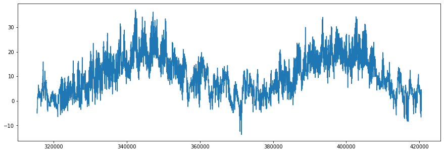
test_series.plot()
plt.show()

LightGBM¶

import lightgbm as lgb

model = lgb.LGBMRegressor()

model.fit(train_x, train_y,
          eval_metric = 'l1', 
          eval_set = [(val_x, val_y)],
          early_stopping_rounds = 100,
          verbose = 0)

---------------------------------------------------------------------------
OSError                                   Traceback (most recent call last)
<ipython-input-8-f986c650d534> in <module>
----> 1 import lightgbm as lgb
      2 
      3 model = lgb.LGBMRegressor()
      4 
      5 model.fit(train_x, train_y,

~/opt/anaconda3/envs/atsa/lib/python3.7/site-packages/lightgbm/__init__.py in <module>
      6 from __future__ import absolute_import
      7 
----> 8 from .basic import Booster, Dataset
      9 from .callback import (early_stopping, print_evaluation, record_evaluation,
     10                        reset_parameter)

~/opt/anaconda3/envs/atsa/lib/python3.7/site-packages/lightgbm/basic.py in <module>
     41 
     42 
---> 43 _LIB = _load_lib()
     44 
     45 

~/opt/anaconda3/envs/atsa/lib/python3.7/site-packages/lightgbm/basic.py in _load_lib()
     32     if len(lib_path) == 0:
     33         return None
---> 34     lib = ctypes.cdll.LoadLibrary(lib_path[0])
     35     lib.LGBM_GetLastError.restype = ctypes.c_char_p
     36     callback = ctypes.CFUNCTYPE(None, ctypes.c_char_p)

~/opt/anaconda3/envs/atsa/lib/python3.7/ctypes/__init__.py in LoadLibrary(self, name)
    440 
    441     def LoadLibrary(self, name):
--> 442         return self._dlltype(name)
    443 
    444 cdll = LibraryLoader(CDLL)

~/opt/anaconda3/envs/atsa/lib/python3.7/ctypes/__init__.py in __init__(self, name, mode, handle, use_errno, use_last_error)
    362 
    363         if handle is None:
--> 364             self._handle = _dlopen(self._name, mode)
    365         else:
    366             self._handle = handle

OSError: dlopen(/Users/prince.javier/opt/anaconda3/envs/atsa/lib/python3.7/site-packages/lightgbm/lib_lightgbm.so, 6): Library not loaded: /usr/local/opt/libomp/lib/libomp.dylib
  Referenced from: /Users/prince.javier/opt/anaconda3/envs/atsa/lib/python3.7/site-packages/lightgbm/lib_lightgbm.so
  Reason: image not found

forecast = model.predict(test_x)
print('  LightGBM MAE: %.4f' % (np.mean(np.abs(forecast - test_y))))

#series[-test_size:].plot(marker = 'o', linestyle = '--')
#plt.plot(forecast, marker = 'o', linestyle = '--')
#plt.show()

  LightGBM MAE: 0.5319

### HYPERPARAMETERS ###
window_size = 240
prediction_horizon = 24

### TRAIN TEST VAL SPLIT ###
train_series = series.iloc[:35045, 1]
val_series = series.iloc[35045:52569, 1]
test_series = series.iloc[52569:, 1]

train_x, train_y = create_xy(train_series.to_numpy(), window_size, prediction_horizon)
val_x, val_y = create_xy(val_series.to_numpy(), window_size, prediction_horizon)
test_x, test_y = create_xy(test_series.to_numpy(), window_size, prediction_horizon)

print(train_x.shape)
print(train_y.shape)
print(val_x.shape)
print(val_y.shape)
print(test_x.shape)
print(test_y.shape)

(34782, 240)
(34782, 24)
(17261, 240)
(17261, 24)
(17260, 240)
(17260, 24)

### LightGBM

recursive_x = test_x
forecast_ms = []
for j in range(prediction_horizon):
    pred = model.predict(recursive_x)
    recursive_x = np.hstack((recursive_x[:, 1:], pred[:, np.newaxis]))
    forecast_ms.append(pred)
forecast_ms = np.asarray(forecast_ms).T
print('LightGBM')
print('MAE:', np.mean(np.abs(test_y - forecast_ms)))
print('RMSE:', np.sqrt(np.mean((test_y - forecast_ms)**2)))
print('')

### Naive

tmp = test_y[:-1, -1]
n_forecast = []

for val in tmp:
    n_forecast.append(np.repeat(val, 24))
n_forecast = np.asarray(n_forecast)

print('Naive')
print('MAE:', np.mean(np.abs(test_y[1:, :] - n_forecast)))
print('RMSE:', np.sqrt(np.mean((test_y[1:, :] - n_forecast)**2)))
print('')


### S.Naive

new_test = np.vstack(np.array_split(test_series.to_numpy()[3:], 730))

print('Seasonal Naive')
print('MAE:', np.mean(np.abs(new_test[1:, :] - new_test[:-1, :])))
print('RMSE:', np.sqrt(np.mean((new_test[1:, :] - new_test[:-1, :])**2)))

LightGBM
MAE: 2.083323119819872
RMSE: 2.7826767013777443

Naive
MAE: 3.184767754022055
RMSE: 4.457663461439199

Seasonal Naive
MAE: 2.613232738911751
RMSE: 3.4171095400347133

Summary¶

Using LightGBM with a recursive forecasting strategy demonstrates that we can achieve an MAE of about 2.08°C without hyperparameter tuning.

Hyperparameter Tuning (Supplementary Notebook) Datasets

By students of PhD in Data Science Batch 2023 at the Asian Institute of Management
© Copyright 2020.

</html>

59 KiB Raw Blame History Unescape Escape

Time Series Analysis Handbook

Temperature Forecasting (Supplementary Notebook)¶

1. Jena Climate Dataset¶

LightGBM¶

Summary¶

59 KiB

Raw Blame History